Core Components of CH
Node Contraction
We introduce the concept of node contraction:
The Idea
When we contract a node, we first remove it from the graph. If the contracted node existed on the shortest path between two of its neighbors before contraction, we add a shortcut edge between the two neighbors such that all shortest path lengths are still preserved.
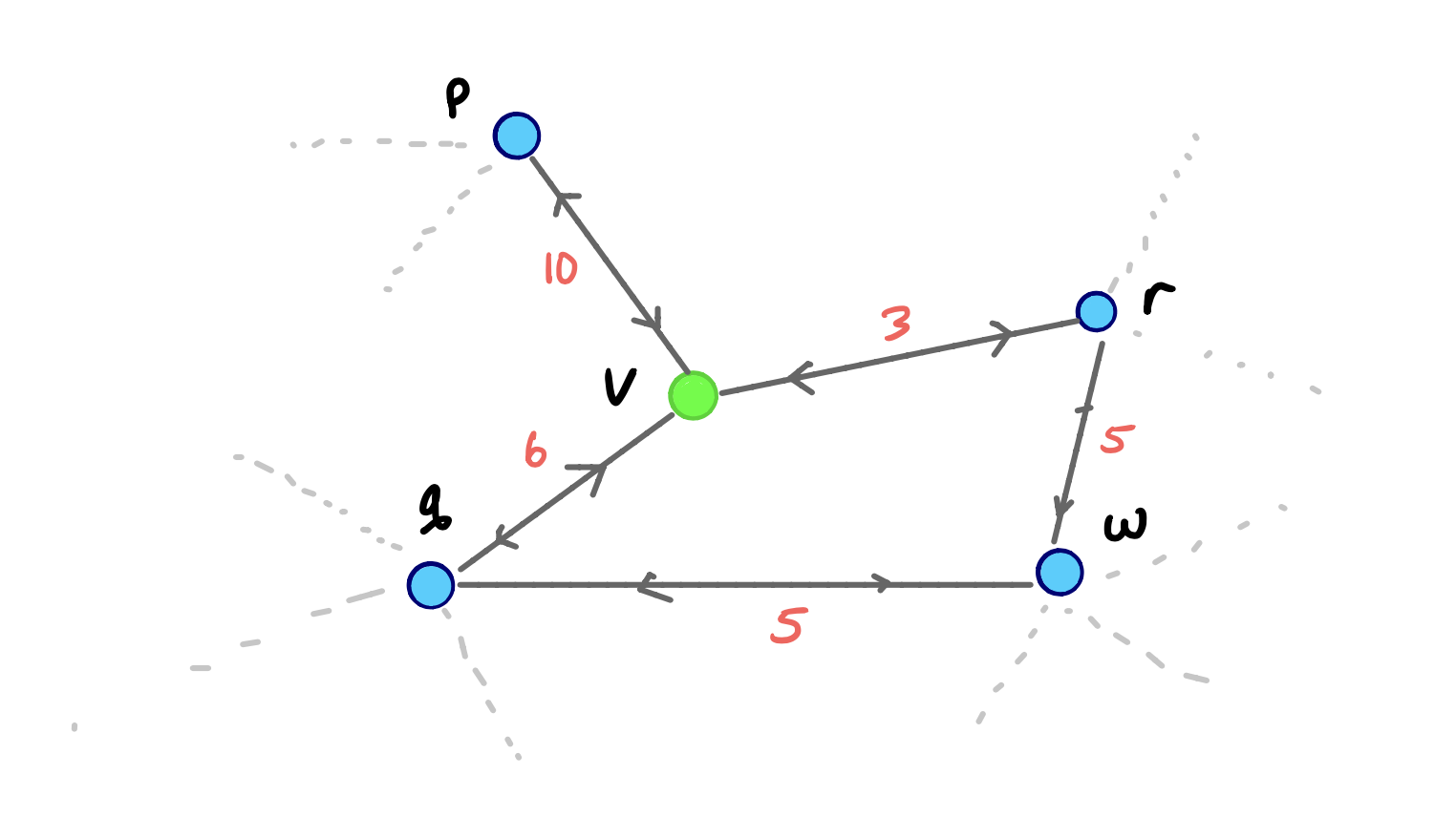
Consider this small example, where we contract node v. We can assume that no other edges exist between v, p, q, and r, other than the ones shown.
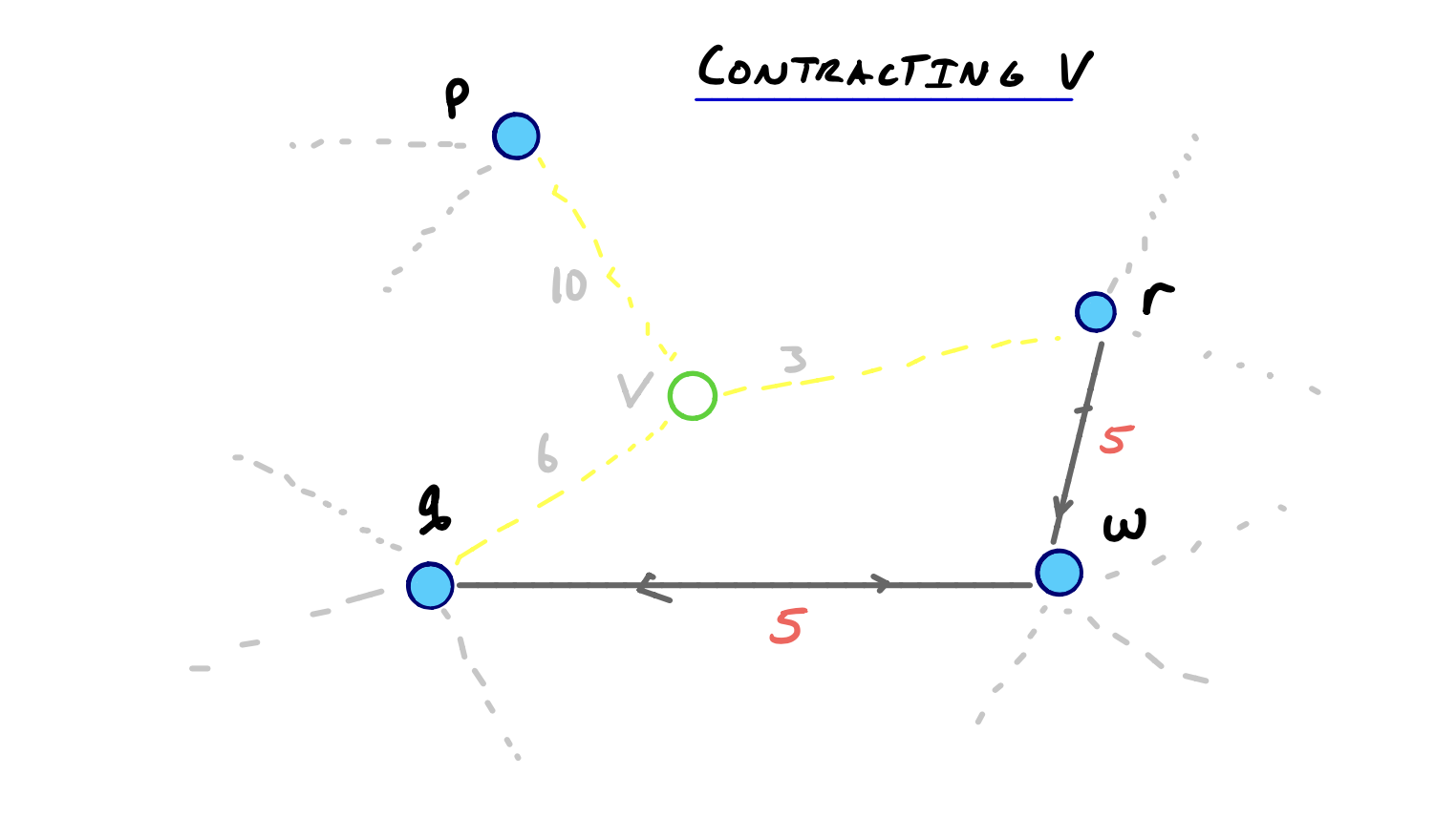
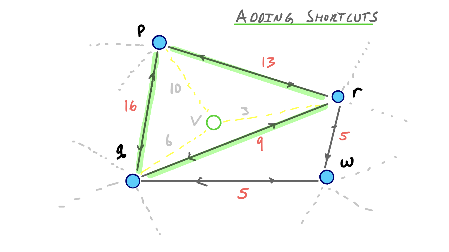
First v and its adjacent edges are dropped from the graph. Then we check if any shortest paths between two neighbors of v actually went through v. In this case, the shortest paths between p and r, q and r, and p and q all used v, so we add the shortcut edges pr, qr, and pq with corresponding weights.
Notice that even though a path from q to r still existed after removing v and its incident edges, it wasn’t the shortest path from q to r, so our shortcut edge qr is needed.
Formal Definition
Consider a node v and the following contract process:
We denote the set of all vertices with edges incoming to v as U, and the set of all vertices with incoming edges from v as W.
Then for each pair of vertices (u, w), for u in U and w in W:
If the path <uvw> is the unique shortest path from u to w, we add a shortcut edge uw to the graph with weight w(u, v) + w(v, w).
Then, we remove v and all of its adjacent edges from the graph.
We’re now done contracting v.
Contraction of All Nodes
Given the concept of node contraction, the CH algorithm tells us to contract each node based on some node ordering.
For now, let’s assume that the ordering has already been established. As you might begin to realize, a good node ordering is the most critical (and expensive) component of a fast CH algorithm, but we’ll also later prove that any ordering of nodes will lead to a correct bidirectional query.
But to illustrate the proces of contracting each node in order, consider that we’ve already ordered our nodes according to some level of importance.
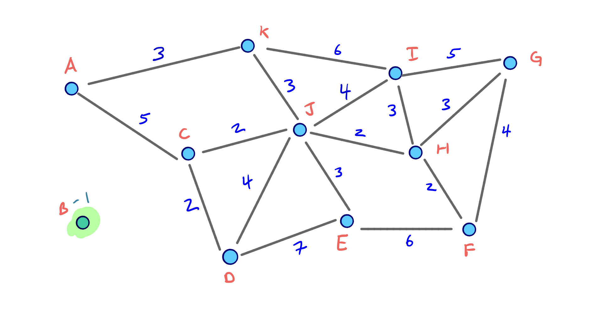
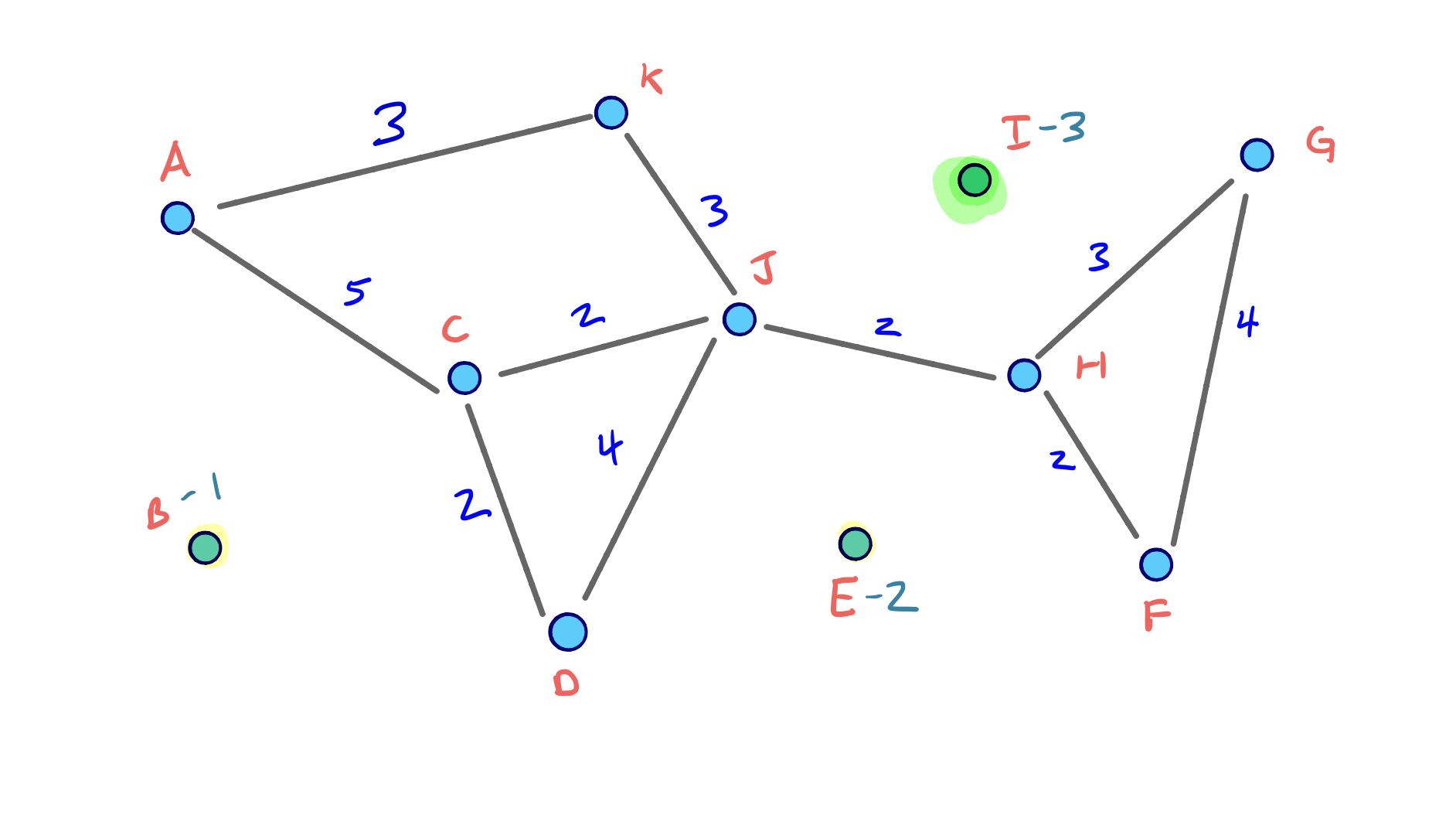
Then, at each iteration i from [1, n] we contract vertex vi by removing vi and all of its adjacent edges from the graph, and we add in any needed shortcut edges.
In iteration i+1, our graph will only have n-i nodes, but it will include any shortcut edges added from previous rounds.
When a node with adjacent shortcut edges is contracted, we also remove its shortcut edges from the graph.
The Overlay Graph
After contracting node vn we consider the overlay graph G* that contains all original nodes and edges and all shortcut edges added during the contraction process.
We use G* for our bidirectional Dijkstra searches.
Example
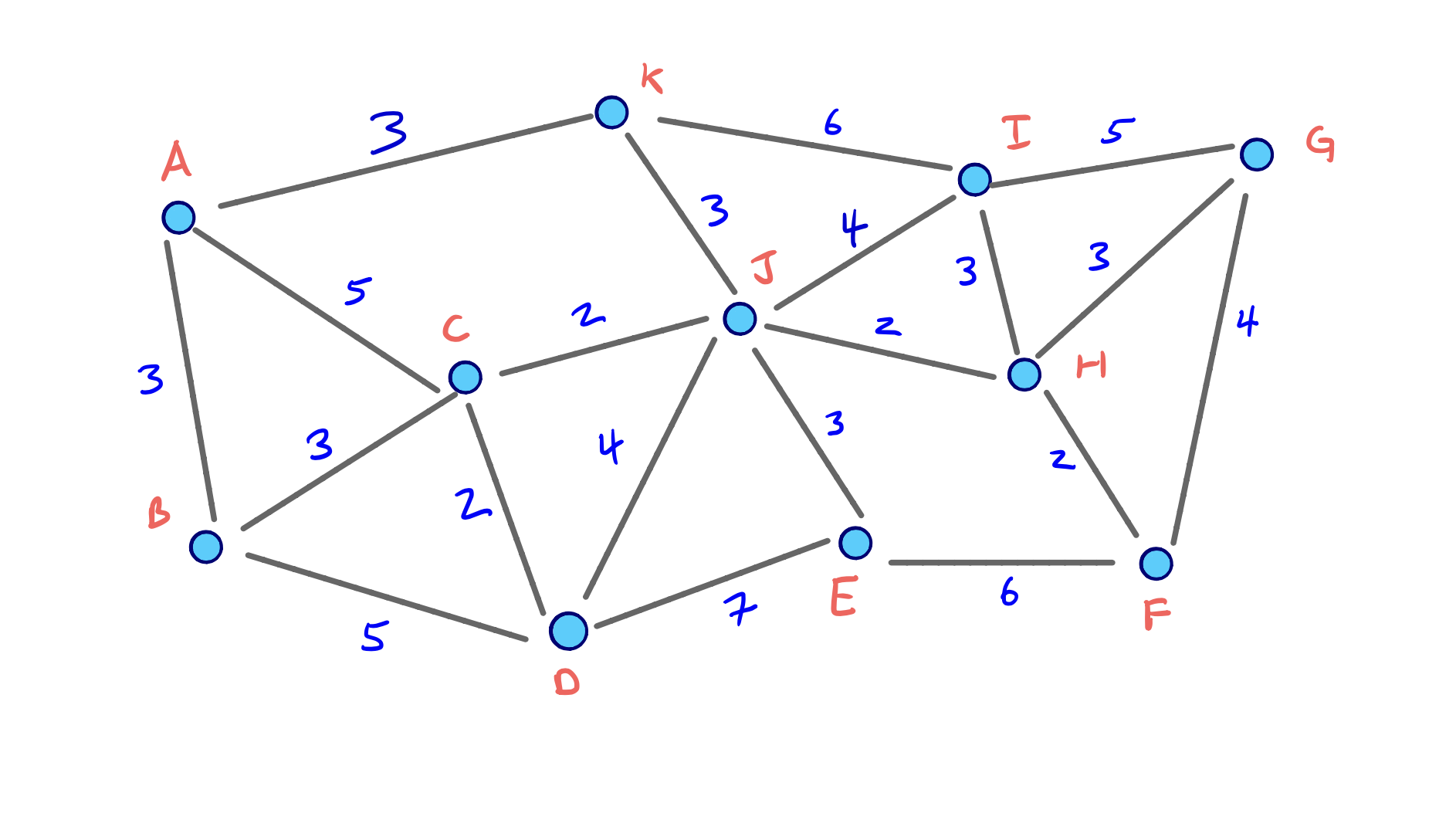
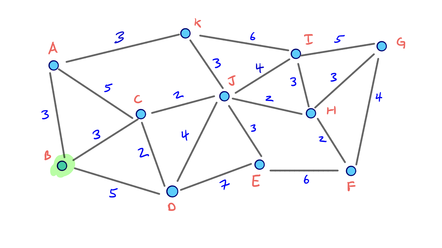
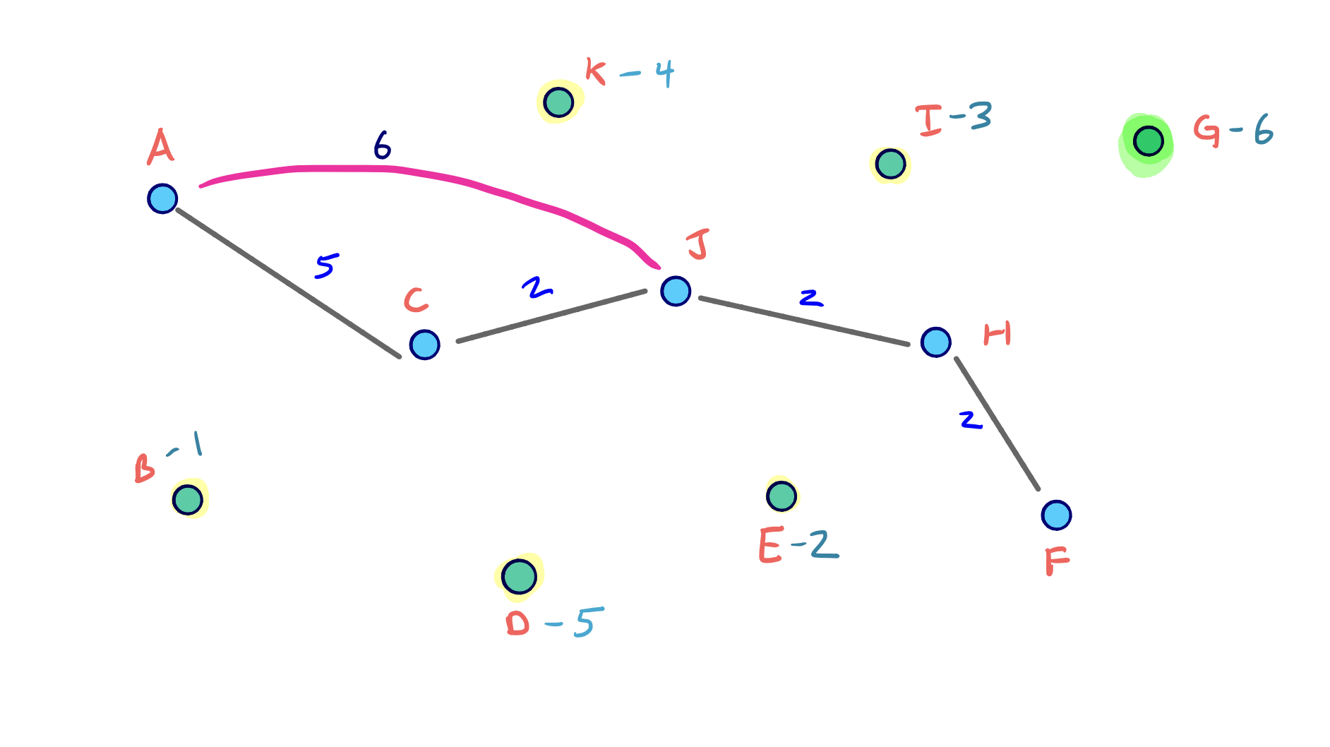
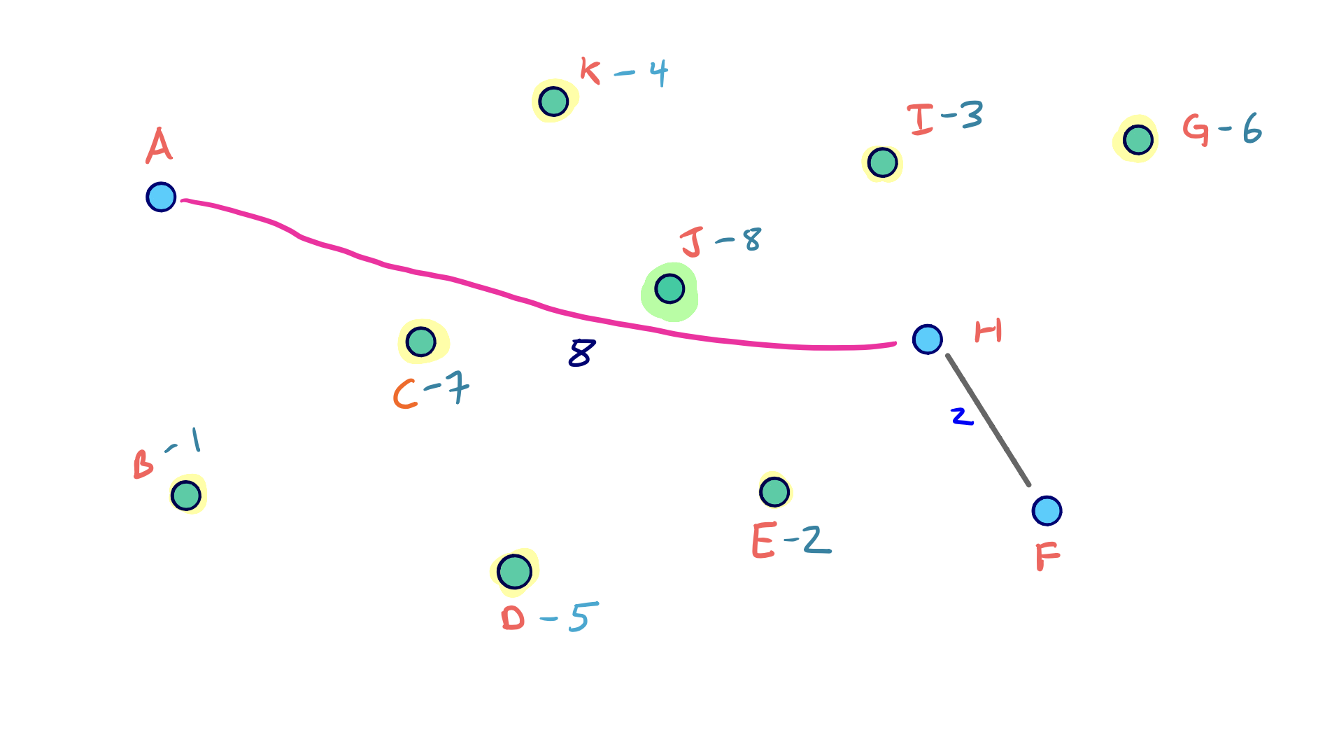
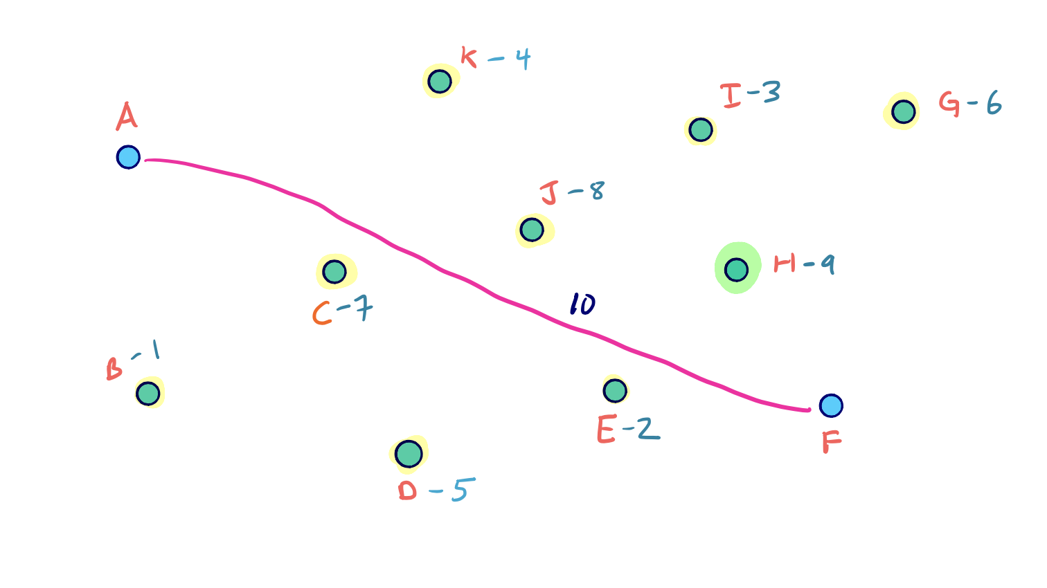
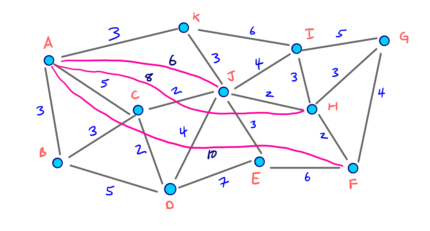
To visualize the full node contraction process, consider the following example graph with an arbitrary node ordering.
We can click through the slides to see the full process:

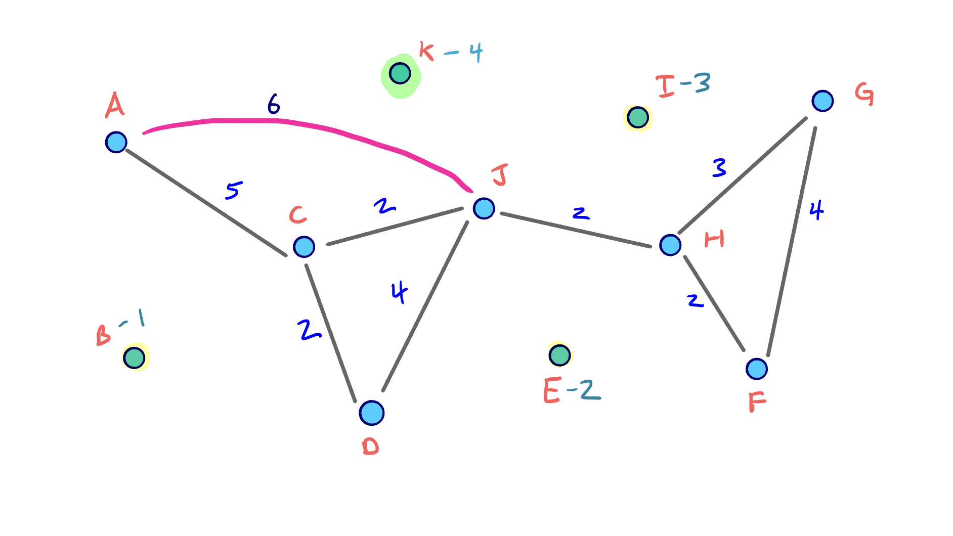


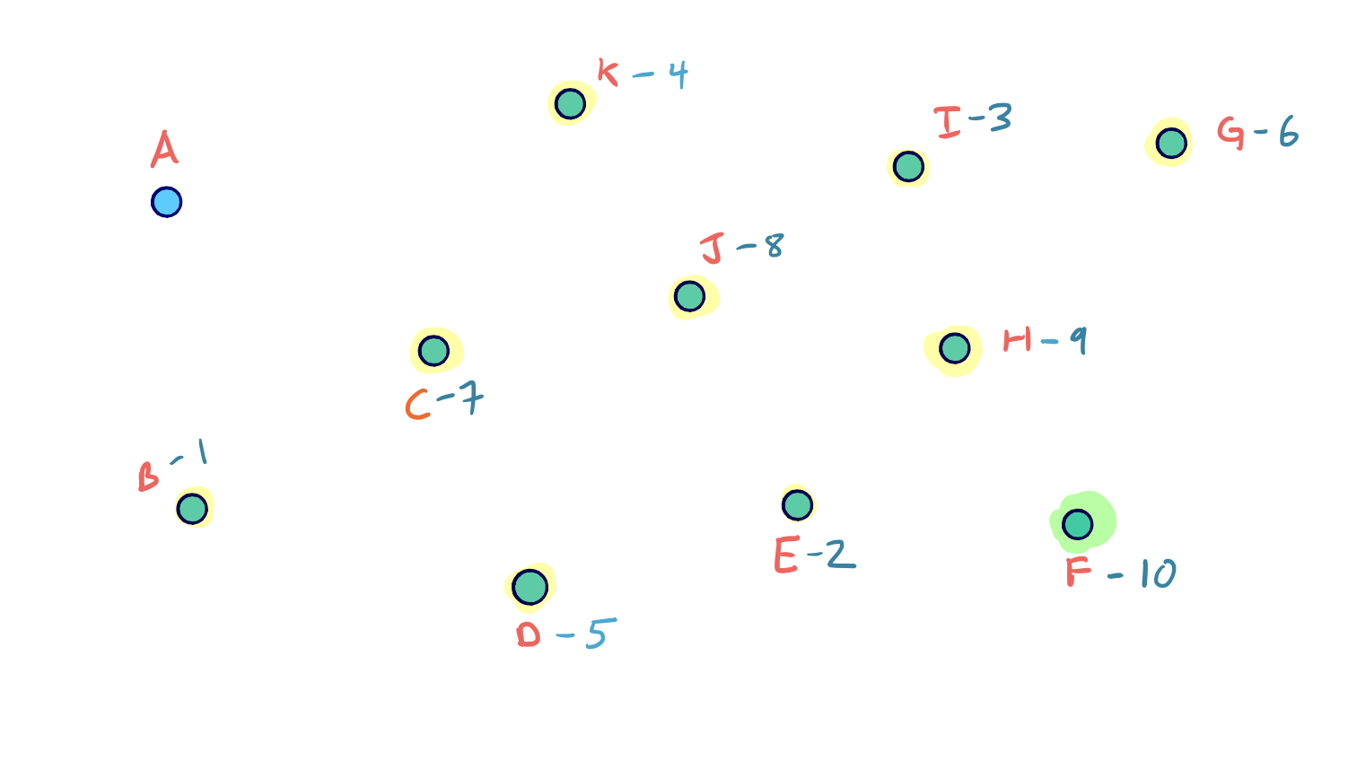

Given this contraction, we can construct and visualize the final G* overlay graph that contains the original graph G with the three shortcuts we added:
You can see that each of the shortcuts preserves the true shortest path structure. Also, depending on our order of node contraction, different shortcut edges could have been added (and we discuss this key component later on).
But for the moment, realize that our ordering was fairly good given that only 3 shortcuts needed to be added.
Efficiently Computing Shortcuts to Add
For our small example graph, it’s relatively easy to eyeball when a node that’s being contracted is on the shortest path between two of its neighbors.
But in general, we need a method for efficiently determining when to add a shortcut edge. We discuss this in the next section.