Core Components of CH
Choosing a Node Order
Our query is correct no matter the order in which nodes were contracted, but a good node ordering has major implications for the performance of the queries. The order in which nodes are contracted affects the shortcut edges that do or don’t get added in G*. And as it’s been mentioned before, too many shortcut edges means too dense a G* graph and slower queries as a result.
So a primary concern with contraction hierarchies is determining a good node ordering during the preprocess step. In turns out that finding an optimal node ordering is hard (see [5]). A lot of continued research and developments to contraction hierarchies deals with finding better heuristics for good node ordering. However, the approaches given by [8] do perform very well in practice.
Strategies for Node Ordering
The general idea is that every node has some cost associated to being contracted, and we want our nodes ordered from least costly to most costly. We can think of cost as a proxy for ‘importance’ as we originally discussed.
It turns out that the main function used to determine this cost involves simulating the contraction of each node. Given that all edges incident to a node are removed during contraction, we’re interested in the edge difference of a node, which is the difference between the number of original edges removed and the number of shortcut edges added.
Let’s revisit our example graph:
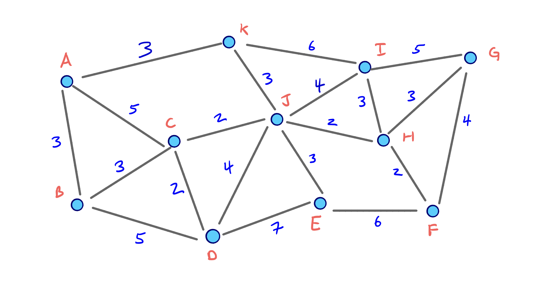
Using our original, arbitrary node ordering, we only added 3 shortcut edges. In the example, B was the first node we contracted, and it didn’t require any shortcuts to be added. In other words, the edge difference of B is -3.
But what if we had first contracted J first? Compare what choosing J over B looks like:


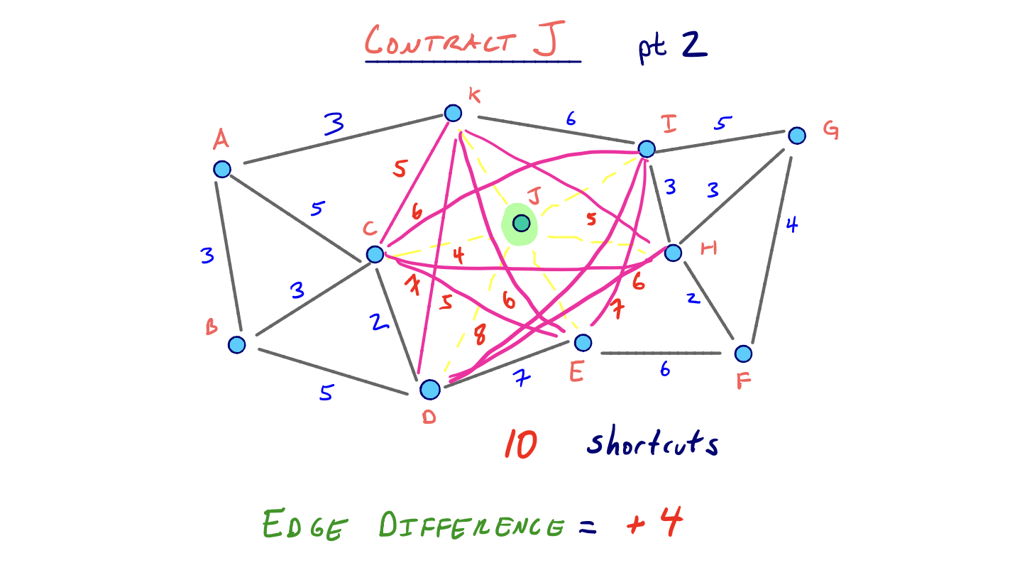
So clearly J has a much greater edge difference than B, and so J is less attractive to contract early on. Nodes like J are hubs that connect many of its neighbors with low costing edges. Its adjacent edges are like highways that should be used in the middle of long trips, just as the shortest path from B to G did. So it would make sense that a node like J is important and shouldn’t be contracted early on if we want the best possible query performance.
Computing the Order and Contracting All Nodes
Then a primary method for determining a node order and subsequently contracting all nodes in that order involves maintaining a priority queue based on some cost function, which in our case is simply the edge difference of each node.
So first, to load the priority queue, we can compute the edge difference of each node by simulating its contraction. Given what we know about computing shortcuts, we’re doing a constant amount of work per node, which initially gives us a linear amount of work for this step.
But consider that after we begin contracting nodes, the edge difference for other nodes can be affected. If we wanted to strictly adhere to an ordering based on edge difference, we would need to recompute the edge difference for every remaining node in the graph after each contraction. Of course, this would end up taking quadratic time, so it isn’t feasible. Instead, we can use the lazy update heuristic proposed by [9].
Lazy Updating
To use this heuristic, consider that we’ve already computed our initial node ordering. Now we’re in the process of actually contracting each node in order, by extracting the min from our priority queue.
Before contracting the next minimum node, we recompute its edge difference. If it’s still the smallest in the priority queue, we can go ahead and actually contract it. If its edge difference is no longer the min, then we update its cost and rebalance our PQ. We then check the next minimum node and continue this process. [8] and [9] find that performing these lazy updates results in improved query times because of a better, updated contraction order.
Other heuristics used to update the cost values in the priority queue involve only recomputing edge differences for neighbors of the most recently contracted node. We could also decide to do a full re-computation of edge differences for all remaining nodes if too many lazy updates occur in successive order.
Other Cost Functions
Additionally, we can consider other factors to determine the cost of contraction. For example, we might consider the idea of uniformity to be important when contracting nodes. This means varying the location of nodes in terms of their contraction order.
Conceptually, we wouldn’t want to contract all nodes in a small region of the graph consecutively because we could risk adding too many wasteful shortcuts. In our original example, we had a pretty good ordering partly because nodes in different parts of the graph were contracted each round.
So an additional term to consider is the number of contracted neighbors each node has. This just involves counting the number of neighbors in the original graph that have already been contracted. When dealing with multiple terms like contracted neighbors and edge difference to determine cost, we would use a linear combination of terms.
Advanced Heuristics for Node Order
In the original presentation of contraction hierarchies, [8] and [9] use even more sophisticated terms for determining a node order that are beyond the scope of this site. However, all well-performing orderings use some combination of both edge difference and contracted neighbors. And it should be clear that a tradeoff exists between more involved node orderings that can improve query times, but that may cost more during the preprocess stage.
In sum however, even using the two simple terms we introduced with the lazy update heuristic provide a good foundation.