Core Components of CH
The Modified, Bidirectional Query
So consider now that during our preprocessing stage we:
- Ordered all nodes
- Contracted each node in order
- Have an overlay graph G* containing all original nodes and edges, and also all shortcut edges added during the contraction phase.
Now we want to query our graph to find the shortest path between a source s and a target t.
The CH query uses a modified version of the bidirectional Dijkstra search we introduced earlier, but it considers only smaller subgraphs of G* in both directions. We call these the upward and downward graphs.
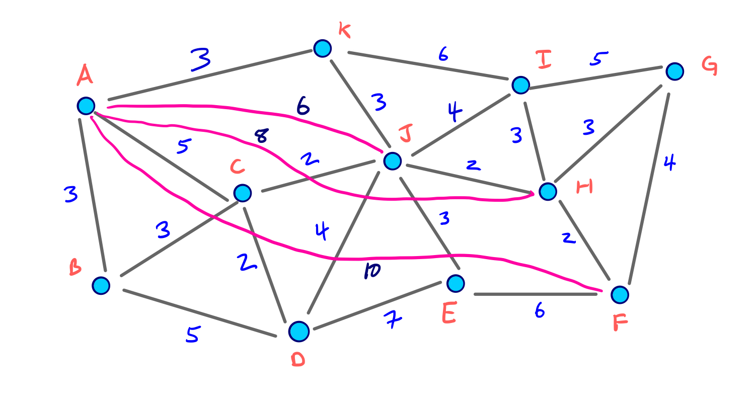
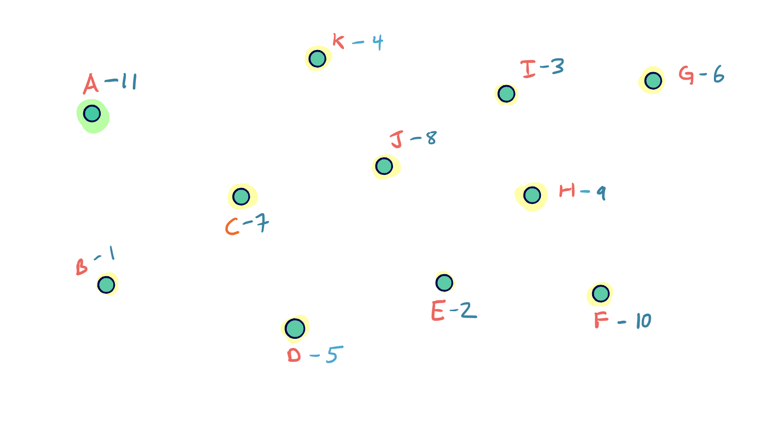
For reference, recall the G* graph from our earlier contraction example. In the second slide we also see the node ordering that we used:
Upward and Downward Graphs
Given our order of nodes, we denote for nodes v and w that v > w if v was contracted after w. And we say that v < w if v was contracted before w.
Then we can define the upward and downward graphs:
The upward graph G*U only contains edges from v to w where v > w.
The downward graph G*D only contains edges from v to w where v < w.
Because every node has a unique position in the ordering, every edge is either in the upward or downward graph.
The Bidirectional Search Spaces
Recall that in the original bidirectional search method, we run a forward search from the source and a backward search from the target. For our CH query from s to t, we run a forward search from s on the G*U graph, and a backward search from t on the G*D graph.
However, for symmetric graphs like the ones we are considering, a backward search (reversing edge directions) on G*D is the same as an upward search on G*U. So from both our source and target nodes, we can perform a standard Dijkstra search on the G*U graph.
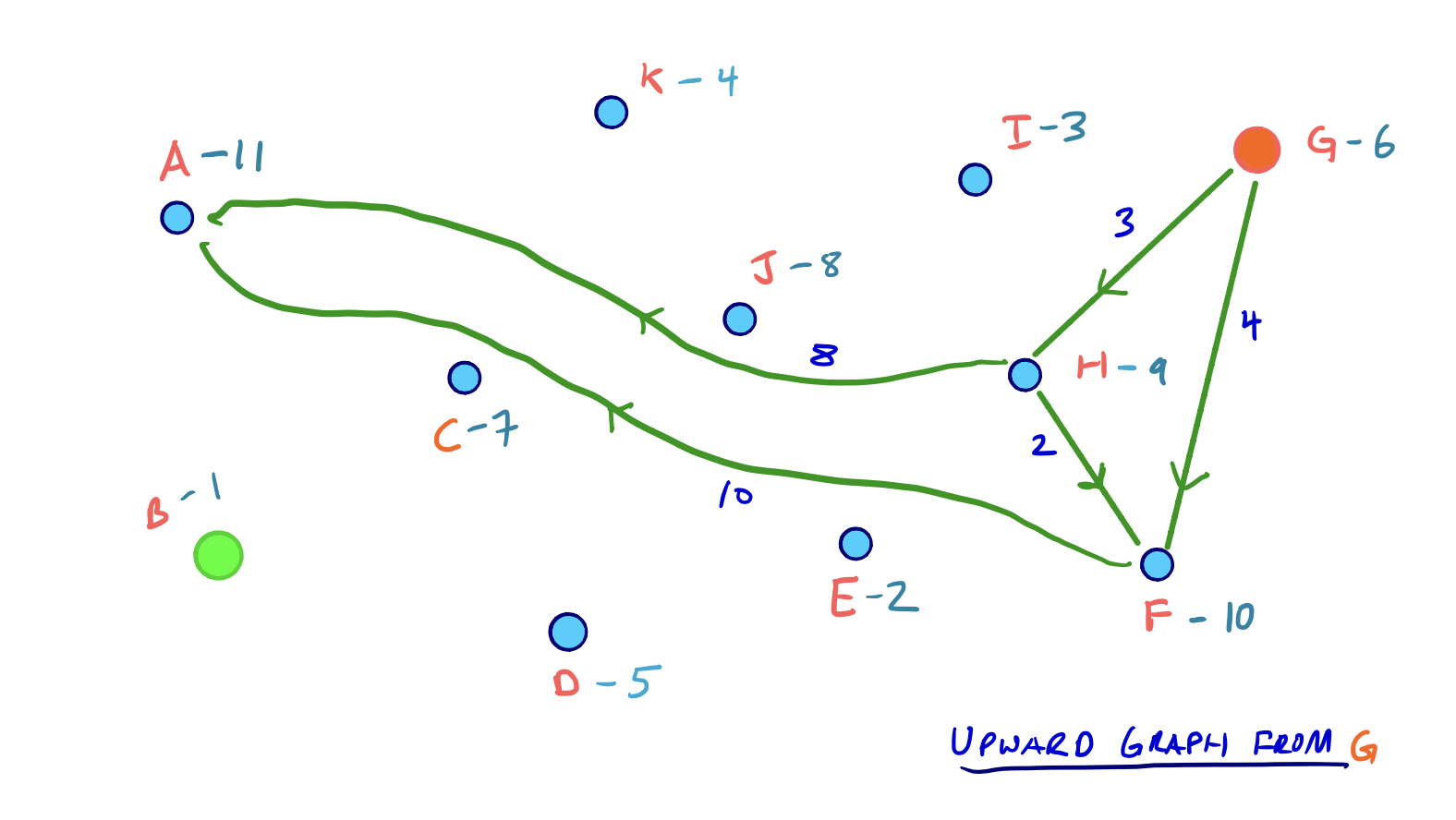
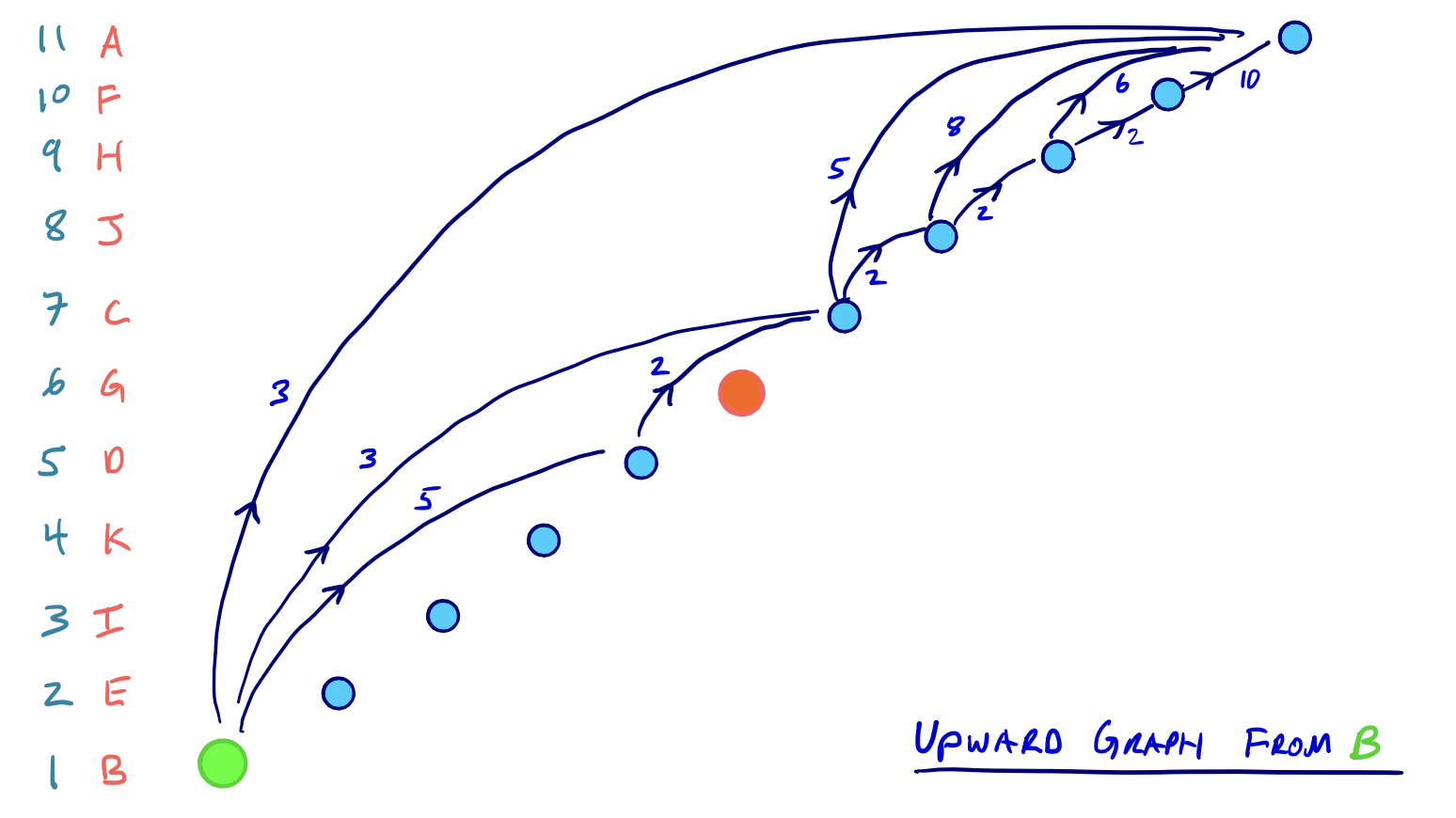
From our example above, let’s say our source node is B and our target node is G. Then the two respective search spaces on G*U will look as follows:
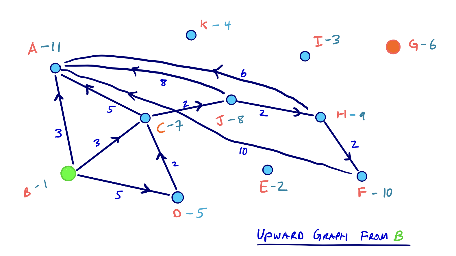
Although we said that every edge in G* is either in the G*U or the G*D graph, not all edges in G*U will be relevant in the search space from a given node.
In our example above, for example, the edge ED does exist in G*U since E was contracted before D. But, because there is no path to E in either of the two searches from B or G, we would never need to consider the edge ED.
Then on both of these upward graphs, we run a complete Dijkstra search, meaning that all nodes in both subgraphs must be settled. And it should be evident that in both searches, the number of settled nodes and relaxed edges is significantly reduced than if we were searching on the entire G* graph.
Moreover, because we have a complete ordering of nodes, the two search spaces can both be conceptualized as DAGs (directed acyclic graphs) and are inherently topologically sorted. Consider the redrawing of the two searches that emphasizes this hierarchical nature of the contraction order:

Implementations of the CH query in [8] and [9] don’t explicitly topologically sort the subgraphs before running the search, but it is a helpful conceptual model.
Finding the Shortest Path Length
In any case, after running two complete Dijkstra searches on G*U from both the source and target, we have a set of nodes that are settled in both searches. We denote this set as L.
Continuing with our example from above, we see the nodes in L shaded in red with their corresponding shortest path scores:
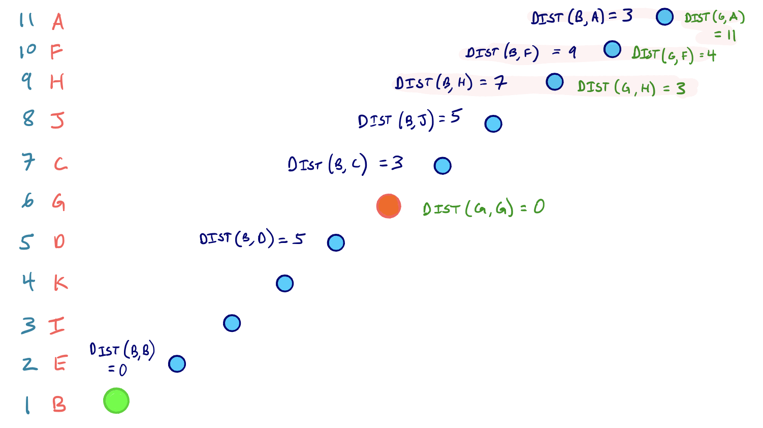
For every node v in L, we sum the shortest path scores of v (one score from s, one from t). The shortest path distance then is the minimum sum over all v in L.
In other words:
dist(s, t) = min{ dist(s, v) + dist(v, t)} over all v in L
So for our source node B and our target node G, the three nodes settled in both searches are H, F, and A. And node H has the scores dist(B,H) + dist(G,H) = 10, which is the smallest sum among the three nodes.
This means the shortest path from B to G is 10 and goes through node H. And we can confirm this from our original G* graph:
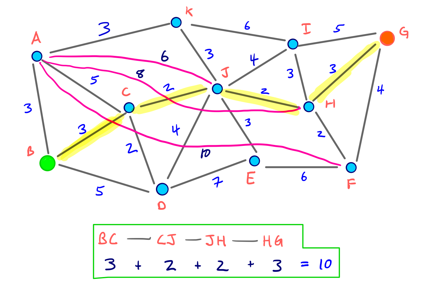
So our modified bidirectional Dijkstra search returns the correct shortest path! And we only relaxed a total of 16 edges during the query, which would compare to 40 relaxations in the original, un-augmented graph.
For this arbitrary example on a small graph the query speedup isn’t huge, but the results on real road networks certainly magnify the extent of the search space reduction.
Unpacking the Actual Shortest Path
We’re able to compute the length of the shortest path, but we still need to unpack the actual arcs used on that path. We can handle this during the stage of contraction when shortcut edges are added. When we add a shortcut edge from u to w during the contraction of v, we store a shortcut pointer to v.
We then begin unpacking the shortest path on the G*U graph from the highest order node, in both directions. We back-trace parent edge pointers as in a regular Dijkstra algorithm, and if the parent edge has a shortcut pointer, we replace the parent edge with the shortcut edge, and continue to recursively unpack the full path.
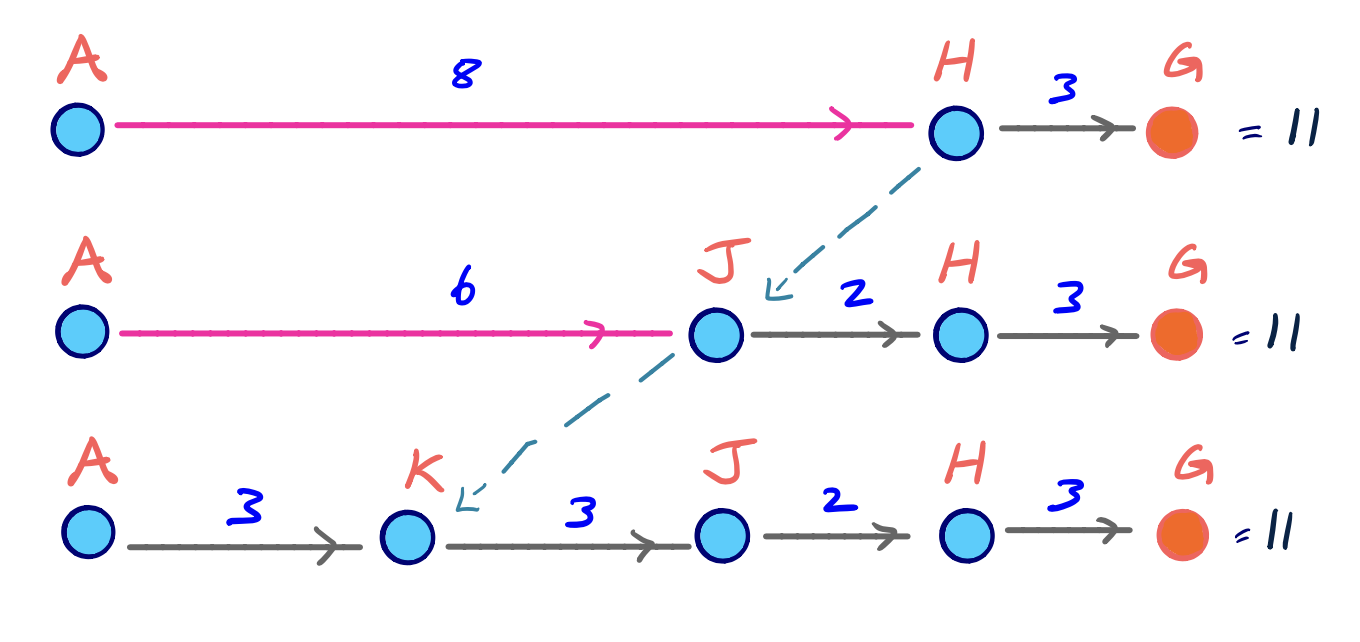
Our example query above didn’t end up using any shortcut edges in G*, but consider if we had queried the shortest path from node A to G. Then, we would certainly use the shortcut edge AH. And since A is the highest-ordered node in terms of contraction time, we can visualize the ‘unpacking’ of shorcut edges as:
Proving Query Correctness
For our example graph, we showed that after the contraction process using our specific node ordering, this query method correctly proved the shortest path between our source and target.
We continue on to show that this query algorithm is correct for any node ordering.